h-Edit: Effective and Flexible Diffusion-Based Editing via Doob's h-Transform

We formulate image editing as a reverse-time bridge modelling problem, constructing a bridge from the source distribution \( p(x_T) \) to a target distribution \( p(x_0)\, p_{\mathcal{Y}}(y \mid x_0) \), where \( p_{\mathcal{Y}}(y \mid x_0) \) quantifies how likely \( x_0 \) possesses the attribute \( y \).

This provides a principled theoretical foundation and ensures samples come directly from the desired distribution—yielding high editing fidelity and faithfulness.

To handle multiple editing types (e.g., text, style), we extend the target distribution: \[ p(x_0)\, p_{\mathcal{Y}}(y_1 \mid x_0)\, p_{\mathcal{Y}}(y_2 \mid x_0)\, \ldots\, p_{\mathcal{Y}}(y_n \mid x_0), \] enabling multiple edits within one unified framework.

A. Overview

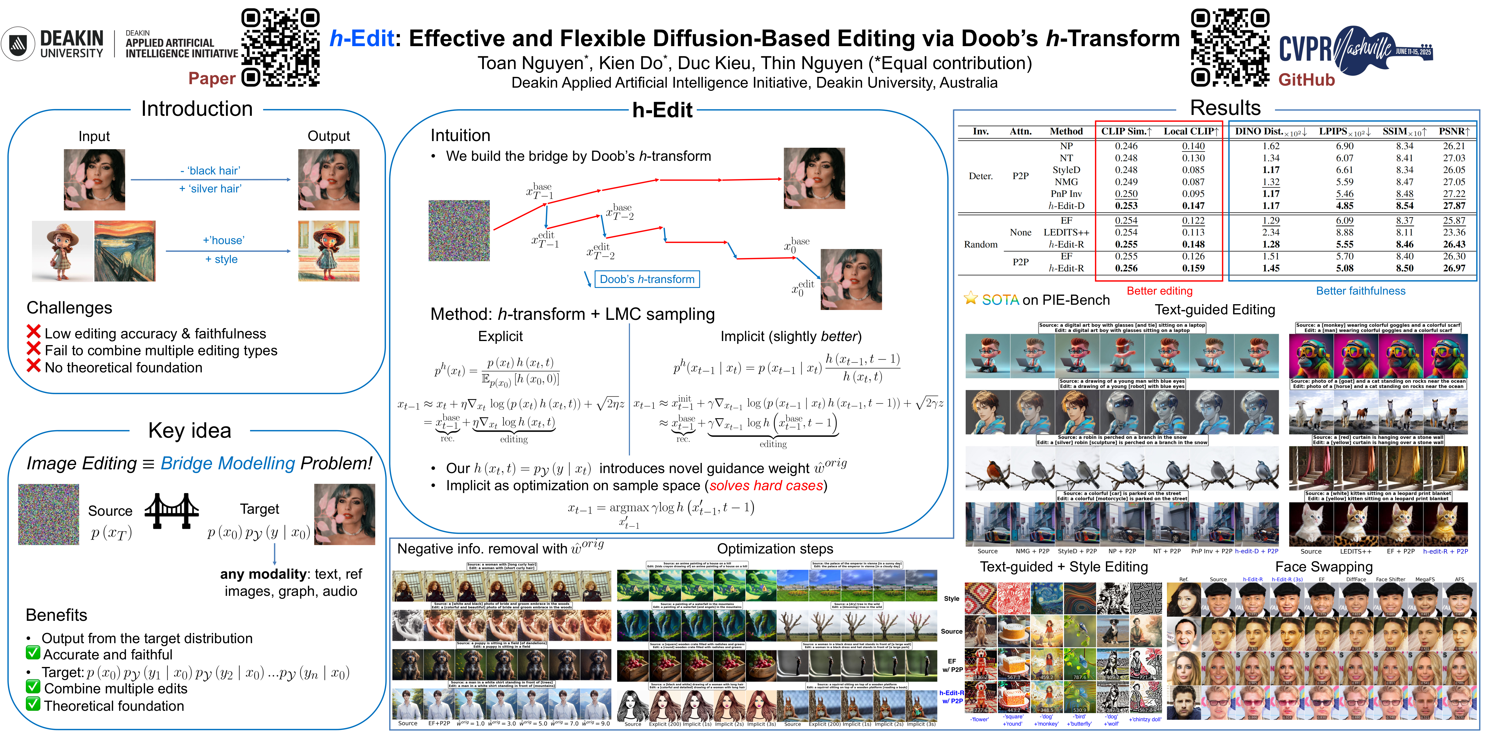
We leverage Doob's h-transform to steer the generative process from a source distribution toward a target distribution that satisfies a desired condition. This is implemented in two complementary forms: implicit and explicit, both enabling flexible guidance without retraining.

Implicit form (slightly better):

We modify the transition distribution \( p(x_{t-1} \mid x_t) \) using the h-transform:

\[ p^{\text{h}}(x_{t-1} \mid x_t) = \frac{p(x_{t-1} \mid x_t)\, h(x_{t-1}, t - 1)}{h(x_t, t)} \] where \( h(x_t, t) = p_{\mathcal{Y}}(y \mid x_t) \) quantifies how likely \( x_t \) possesses the attribute \( y \).

Explicit form:

We modify the marginal distribution \( p(x_t) \) using the h-transform:

\[ p^{\text{h}}(x_t) = \frac{p(x_t)\, h(x_t, t)}{\mathbb{E}_{p(x_0)}[h(x_0, 0)]} \]

As shown in our paper, adjusting \( p(x_{t-1} \mid x_t) \) and \( p(x_t) \) in this manner helps the process converge toward the desired target distribution at the final time step.

Sampling: To generate the next sample \( x_{t-1}^{\text{edit}} \), we apply Langevin Monte Carlo (LMC) sampling in both cases:

• In the implicit form, we sample from \( p^{\text{h}}(x_{t-1} \mid x_t) \)
• In the explicit form, we use the score \( \nabla_{x_t} \log p^{\text{h}}(x_t) \)

B. Update Formulations

Explicit Form:

We perform a direct update using the score of the modified marginal distribution:

\[ \begin{aligned} x_{t-1} &\approx x_t + \eta \nabla_{x_t} \log \left( p(x_t)\, h(x_t, t) \right) + \sqrt{2\eta}\, z \\ &= \underbrace{x_{t-1}^{\text{base}}}_{\text{rec.}} + \underbrace{\eta \nabla_{x_t} \log h(x_t, t)}_{\text{editing}} \end{aligned} \]

Key Advantage of Explicit Form: The update naturally decomposes into a reconstruction term and an editing term. This allows incorporating multiple editing objectives by simply adding more h-functions.

Implicit Form:

We update \( x_{t-1} \) using the gradient of the modified transition distribution:

\[ \begin{aligned} x_{t-1} &\approx x_{t-1}^{\text{init}} + \gamma \nabla_{x_{t-1}} \log p^{\text{h}}(x_{t-1} \mid x_t) + \sqrt{2\gamma}\, z \\ &= \underbrace{x_{t-1}^{\text{base}}}_{\text{rec.}} + \underbrace{\gamma \nabla_{x_{t-1}} \log h(x_{t-1}^{\text{base}}, t-1)}_{\text{editing}} \end{aligned} \]

Key Advantage of Implicit Form: The update can be framed as an optimization problem over \( x_{t-1} \), enabling iterative refinement:

\[ \begin{aligned} x_{t-1}^{(0)} &= x_{t-1}^{\text{base}} \\ x_{t-1}^{(k+1)} &= x_{t-1}^{(k)} + \gamma \nabla_{x_{t-1}} \log h(x_{t-1}^{(k)}, t - 1) \end{aligned} \]

✅ Especially effective for hard editing cases (see experiments).

C. Designing h-Formulations

C.1. Text-Guided Editing Design

We compute the gradient of the h-function as:

\[ \begin{aligned} \nabla \log h(x_{t-1}, t - 1) &= \nabla \log p(y \mid x_{t-1}) \\ &= \nabla \log p(x_{t-1} \mid y) - \nabla \log p(x_{t-1}) \end{aligned} \]

Where: \[ \nabla \log p(x_{t-1} \mid y) = \frac{-\tilde{\epsilon}_\theta(x_{t-1}, t - 1, c^{\text{edit}})}{\sigma_{t-1}}, \quad \nabla \log p(x_{t-1}) = \frac{-\tilde{\epsilon}_\theta(x_{t-1}, t - 1, c^{\text{orig}})}{\sigma_{t-1}} \]

We use classifier-free guidance to compute \( \tilde{\epsilon}_\theta \) as follows:

\[ \begin{aligned} \tilde{\epsilon}_\theta(x_{t-1}, t - 1, c^{\text{edit}}) &= (1 - w^{\text{edit}})\, \epsilon_\theta(x_{t-1}, t - 1, \varnothing) + w^{\text{edit}}\, \epsilon_\theta(x_{t-1}, t - 1, c^{\text{edit}}) \\ \tilde{\epsilon}_\theta(x_{t-1}, t - 1, c^{\text{orig}}) &= (1 - \hat{w}^{\text{orig}})\, \epsilon_\theta(x_{t-1}, t - 1, \varnothing) + \hat{w}^{\text{orig}}\, \epsilon_\theta(x_{t-1}, t - 1, c^{\text{orig}}) \end{aligned} \]

✅ The weight \( \hat{w}^{\text{orig}} \) (different from \( w^{\text{orig}} \) used in the inversion process) plays a key role in suppressing negative content in editing while preserving the identity or structure of the original sample (see experiments).

Comparison with other methods:

C.2. Reward-Based Editing

We compute the gradient of the h-function based on rewards defined at the initial step:

\[ \begin{aligned} \nabla \log h(x_{t-1}, t - 1) &= \nabla \log \left[ \sum_{x_0} p(x_0 \mid x_{t-1})\, h(x_0, 0) \right] \\ &= \nabla \log \left[ \mathbb{E}_{p(x_0 \mid x_{t-1})} [h(x_0, 0)] \right] \\ &\approx \nabla \log \left[ h(x_0 \mid x_{t-1}, 0) \right] \end{aligned} \]

Here, \( x_0 \mid x_{t-1} \) is approximated using Tweedie's formula, enabling reward-driven gradients from models trained at timestep 0 to influence editing at later steps. We apply this approach to style transfer using CLIP and face swapping using ArcFace (see experiments).